We get it, there are CAMPing people and there are people who will never go CAMPing. If you're on the fence, this part of the tutorial describes the novel things CAMP can do, and why you should consider CAMPing. If you're already onboard, you can skip this section, pack your bags and move on to Boot CAMP: Part 1 - Box Model.
There are three features of CAMP that set it apart from other approaches to solving chemical systems in atmospheric models. These are its combined solving of gas- and aerosol-phase chemistry and partitioning, its run-time configuration and its portability across models with different ways of representing aerosol systems and different aerosol mircophysical schemes. These features are described in more detail below and are followed by an example of how a chemist doing laboratory experiments on atmospheric systems can use CAMP to rapidly deploy their new chemistry to a suite of atmospheric models.
Combined solving
Typically, chemical systems are spread across several distinct modules within atmospheric models (Fig. 1) These modules have often been developed independently and may require significant modification to incorporate new chemical processes (particularly when these span the gas and condensed phases) or to port the module to a new host model with its own set of existing modules. In addition, when interrelated processes with similar rates are solved in separate modules (like gas-phase reactions whose products partition to the condensed phase and undergo further reaction), artifacts from the separated solving can be introduced.
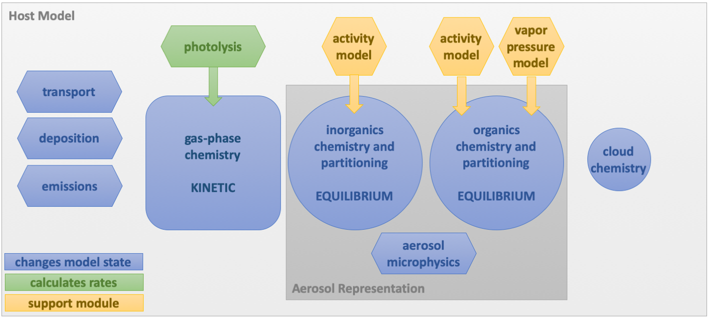
Fig. 1. A typical configuration for chemistry and chemistry-adjacent process in atmospheric models.
CAMP takes a difference approach to solving chemical systems. Instead of solving chemistry across a collection of modules, CAMP accepts rates for processes from modules that would typically directly update the model state (like emissions and deposition), and it uses an object-oriented approach to build an integrated multi-phase chemical system that includes emissions, deposition, gas-phase reactions including photolysis, partitioning between the gas and aerosol phase, and condensed phase reactions in any number of unique aerosol phases (organic, aqueous aerosol, cloud droplets, etc.; Fig. 2). The collection of objects representing the chemistry and related processes are then solved as a single kinetic system, avoiding artifacts from operator splitting and greatly easing the processes of incorporating new multi-phase chemical processes.
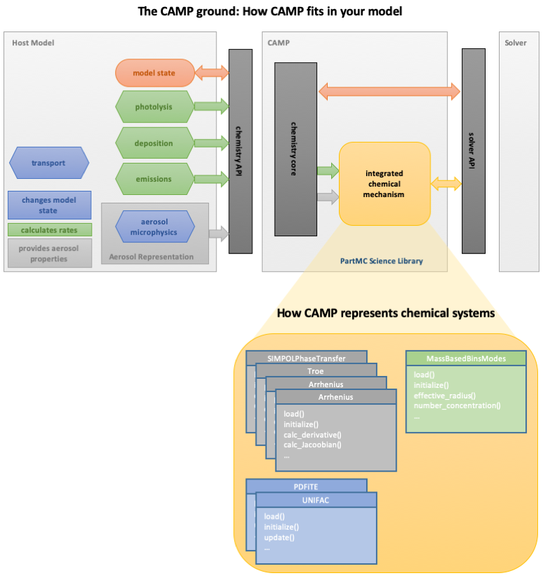
Fig. 2. Schematic showing how CAMP interacts with a host model and how integrated chemical systems are described within CAMP.
We'll see in later parts of the tutorial how these objects are generated and configured, and how CAMP works with the way your model describes aerosol systems (bins, modes, etc.).
Run-time configuration
Another key feature of CAMP is its run-time configurability. As a stand-alone library, you don't need to modify any of the CAMP source code to incorporate CAMP into a new model, but you do need to tell CAMP about the chemical system you want to solve and how your model describes aerosol systems. This is primarily done at run-time using a collection of JSON input files (Fig. 3). (There are also ways to update certain CAMP parameters during a model run, like emissions and photolysis rates.) This opens up many exciting possibilities. To start, you can change the chemical mechanism without any changes to the model source code. Data assimilation and model sensitivity analyses can take advantage of the ability to adjust a wide variety of model parameters (everything from activation energies for Arrhenius reactions to ion-pair interaction parameters in activity calculations) without any changes to source code or recompilation of the model.
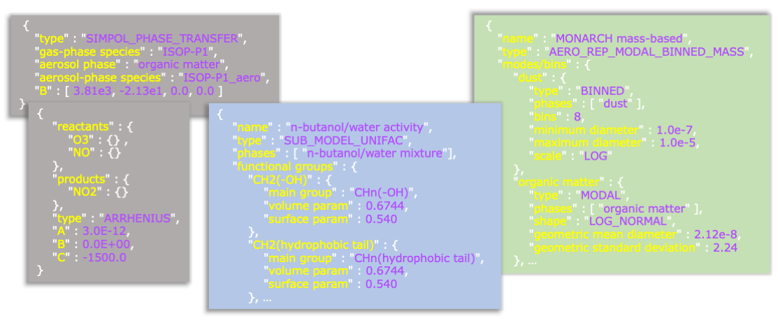
Fig. 3. Examples of JSON input data used with CAMP.
Portability
The last thing we'll mention that makes CAMP unique is its portability across models with different aerosol representations. We'll describe how to make CAMP work with your model's aerosol representation in Boot CAMP: Part 5 - Aerosol Representations. Here, we'll just provide an overview of how CAMP makes this work. Similar to other CAMP model elements, your input data can tell CAMP to create any number of aerosol phases. These are simply collections of species, like an "aqueous" phase that includes "water", "sulfate", "nitrate", etc. Condensed-phase and partitioning reactions must specify the aerosol phase they apply to. Thus, you could have a Henry's law phase transfer reaction for nitric acid that applies to the "aqueous" phase.
The key to separating the chemistry from the host model's aerosol representation is that the chemistry is the same for every instance of a particular aerosol phase, but the number of instances of these phases, and the physical properties of the aerosols of which they are a part, are determined by the host model's aerosol representation. A description of this representation is provided by another JSON input object. This input data specifies not only the type and dimensions of the aerosol representation (e.g., the number and size of bins, or the number and shape of modes) but also which aerosol phases are associated with with which aerosol groups. Some examples of how different aerosol representations implement instances of the same set of aerosol phases in the CAMP state array are shown in Fig. 4.
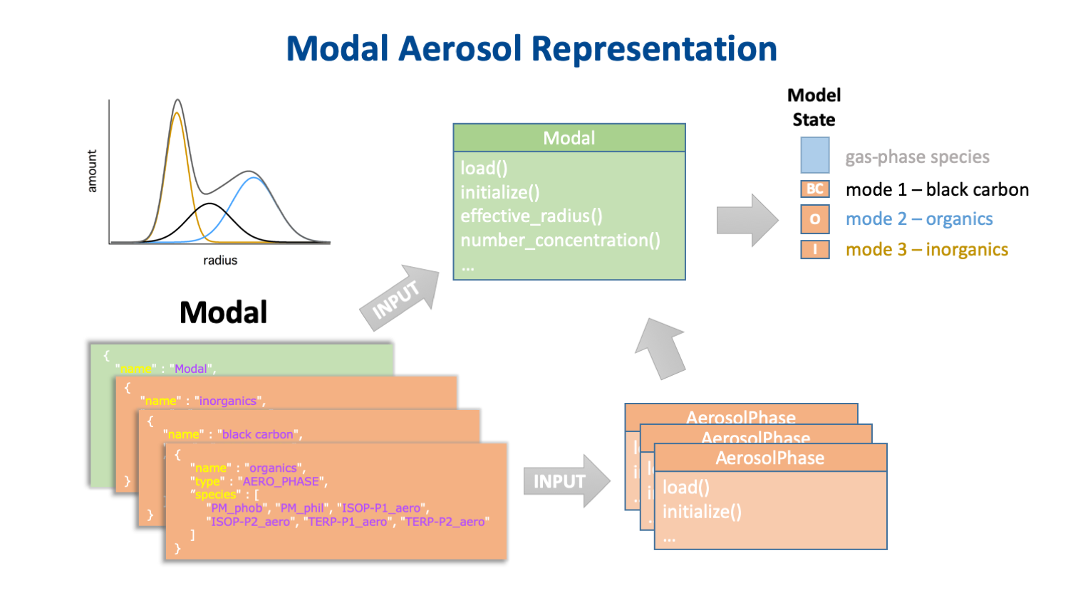
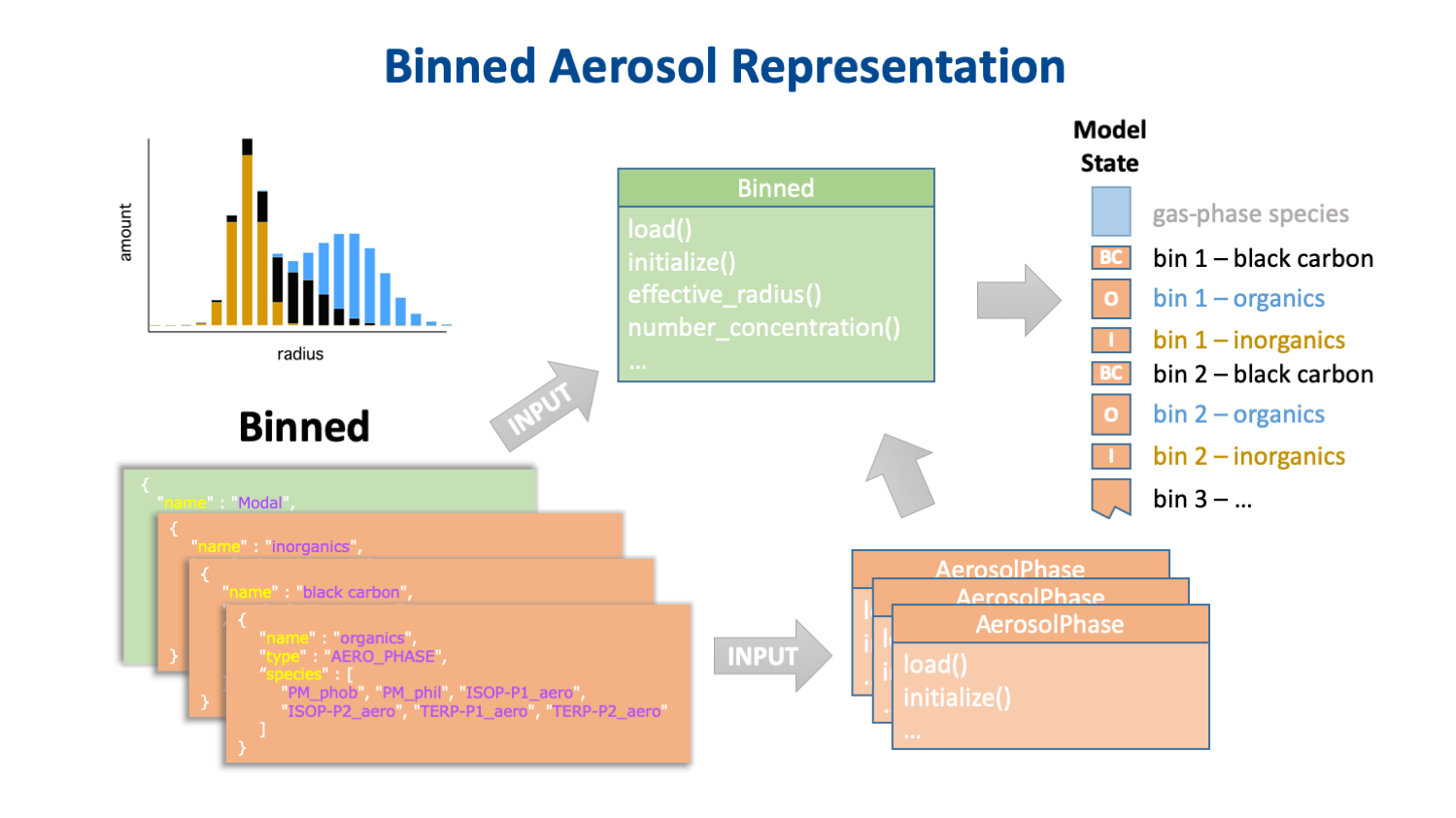
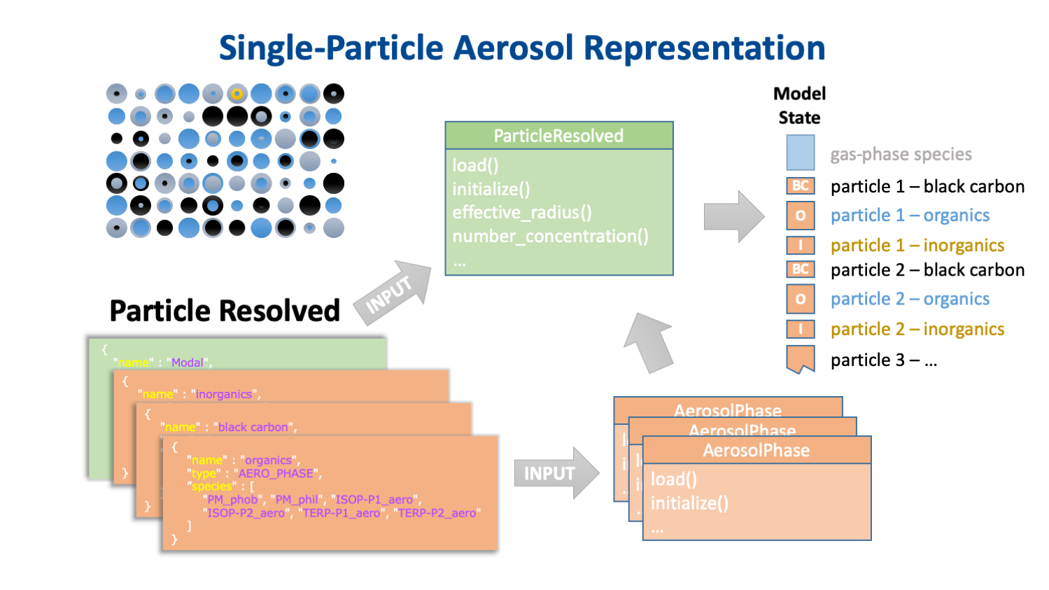
Fig. 4. How modal (top) binned (middle) and single-particle (bottom) aerosol representations might implement the same three aerosol phases.
How you might CAMP
To demonstrate how CAMP functionality can be used in a real-world scenario, imagine you are a reasearch chemist who just discovered a new gas-phase reaction:
\[\ce{ A + OH -> B }\]
Species B can partition to an aqueous phase where it reacts with nitrate:
\[\ce{ B + NO3- -> C }\]
Species C can then repartition back to the gas-phase.
You first try this out in a box model running CAMP with a standard gas and aerosol phase mechansim by adding a single JSON file to the CAMP input file list. Your new file has three chemical species, one gas-phase Arrhenius reaction, one Henry's law phase transfer reaction, and one condensed-phase Arrhenius reaction. The only modification to the existing mechanism input files you make is to add species C to the "aequeous" aerosol phase. You evaluate the model results and tweak the reaction parameters until you're able to fit your experimental results.
Next, you take your mechanism input files and run them in a PartMC particle-resolved urban plume scenario to evaluate the effects of mixing state on your newly discovered system. Then you try out your mechanism in the MONARCH chemical weather prediction system to see the regional and global scale impacts of your new chemistry. What is most important about this process, and what makes CAMP so unique, is that you use the the same input files in all three models and you never modify source code or recompile a model. Your chemistry is running in the exact same version of CAMP in all three models. If that doesn't make you want to try CAMPing, probably nothing will.
So lace-up your hiking boots and stay hydrated. It's time to start the first stage of Boot CAMP!
![]() Index
Index ![]() Next: Boot CAMP: Part 1 - Box Model >
Next: Boot CAMP: Part 1 - Box Model >